CMPSCI 670: Computer Vision, Fall 2014
Homework 5: Recognition (Cats vs. Dogs)
Due date: November 19 (before the class starts)
Overview
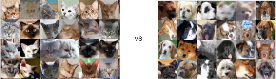
In this homework you will implement various image features and test them using various classifiers on a binary classification task. Images are either of a cat or a dog, and your goal will be to build a classifier that can predict this on unseen images. The relevant material for this homework can be found in lecture 16, 17 and 18.
One of the goals of this homework is to introduce you to recognition benchmarks used in computer vision. The data.zip file has 300 images of cats and dogs. This is a subset of a much larger dataset collected by Omkar Parkhi and others (Oxford-IIIT pet dataset). The original dataset was created to test classification of breeds of cats and dogs, which is even more challenging than our task. Until recently, computer vision algorithms for discriminating cats from dogs were rather poor and this task was even the basis of a CAPTCHA called ASSIRA from Microsoft.
The 300 images are divided into three sets train, val and test. The correct protocol is to tune your parameters for features and classifiers on the train + val set, and then run the classifier on the test set only once. In real benchmarks (or competetions) the test set labels are often withheld. However for convenience the labels for the test set are included in the data.
In this homework you will implement a simple global feature called 'tinyimage' and a bag-of-words feature. You will test these features for classification using k-nearest neighbor (kNN) classifiers and Support Vector Machines (SVMs). Sample implementations of kNN and SVM classifiers are included in the codebase but the parameters for training, such as the k for kNN and lambda (regularization parameter) for SVM have to be set by cross-validation.
You are not expected to match the best results on this task, but produce results that are in the provided range. Your report will be graded on how you explored the space of the design choices. That said, a high accuracy on the test set is a good indicator that your implementation is correct.
Implementation details
After you download the code and data, set the 'dataDir' to the location of the downloaded data, run the evalCode.m. It loads the dataset in a structure called imdb (short for image database). Take a look at various fields in imdb, particularly the list of images, their classId (1=cat, 2=dog), and the imageSet (1=train, 2=val, 3=test). The code right now computes dummy features and evaluates it using a SVM classifier. It obtains an accuracy of 50% on average, just chance performance since half the images are cats. You will improve upon this.
Implement param.feature = 'tinyimage';
Start by implementing a feature called 'tinyimage'. This simply resizes the images to a fixed [n n 3] and makes it a vector of size [1 nxnx3]. Start by setting n = 8 and evaluate the results using kNN classifier ( param.classifier='knn'), and SVM classifier (param.classifier='svm'). You should explore:
- What is the size of the patch that achieves the best classification rate on the validation set.
- What classifier works better for these features?
- What value of k works best for kNN classification?
Implement param.feature = 'bow-patches';
Here you will implement a simple bag of words model where small patches from the image are used as features (implement this inside computeFeatures.m). The key steps to implement this are:- Extract local features from images - write a function that takes a grayscale image and returns a set of grayscale patches of size [2r+1 2r+1] densely sampled from the image. You don't need to extract patches at each pixel, instead sample them uniformly on a grid of locations uniformly spaced 'stride' pixels apart. See the figure below for illustration. Start with r = 8, and stride=12. Thus your local features are tiny grayscale patches of size [17 17] or 289 dimensional features, and there are hundreds of these features in an typical image. Experiment with different values of r and stride, and pick the best one by testing on validation subset.
- Learn a dictionary over the local features. Take a subset of images in the train + val subset and extract several thousands of features from them using the previous step and cluster them using k-means. You don't need to use all the train + val images, but enough to learn a dictionary. A good rule of thumb is to extract at least 100 times more features than the dictionary size you want to learn. A reasonable choice for the dictionary size, i.e., k for your k-means is 128. However, you are welcome to try different values and pick one that leads to best results on the validation set.
- Now you are ready to extract bag of words features. Given an image:
- Extract local features (same as step 1) and assign them to the nearest dictionary items (also called a visual words). You may find the dist2.m file included in the codebase useful which computes all pairs distances between two sets of vectors.
- Build a histogram denoting counts of each visual words.
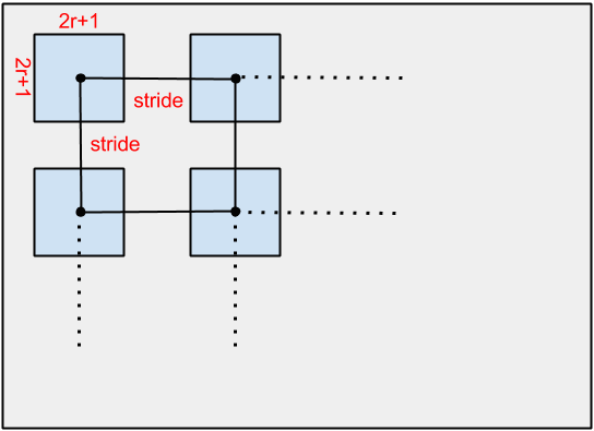
Figure. Extracting dense patches over image. The radius (r) and stride parameter control how these patches are extracted.
Feature normalization - One last step before you can use these features with classifiers is normalization. Each image in the dataset is of a different size which results in different number of visual words per image, hence the histograms are not directly comparable. One way of avoiding this is to normalize the features. You could use either l1-norm, i.e., divide each feature vector by its sum of features, or l2-norm, i.e., divide each feature vector by its length.
Like before, use these features with kNN and SVM classifiers and report results on the validation and test set. Your classifiers should be able to achieve accuracy between 60-70% on the test set, depending on the choices you make about sampling features, dictionary size, radius of the local patch, etc.
Implement param.feature = 'bow-sift';
This is exactly like the previous one, except you use SIFT features. SIFT features are robust to small shifts and illumination changes which are often good traits of a local descriptor. Use the code provided in find_sift.m file to do this. You have to provide a array of locations where you want the SIFT computed and the desired radius of the patch. Like before use a dense sampling of locations. Tune your grid sampling parameter and radius by cross validation. The remaining steps remain exactly the same as before, i.e., instead of local patches, you have SIFT features.
Once again, use these features with kNN and SVM classifiers and report results on the validation and test set. Your classifiers should be able to achieve accuracy between 70-80% on the test set, depending on the choices you make about sampling features, dictionary size, radius of the local patch, etc.
Note: An alternate and faster implementation of kmeans (vl_kmeans) and dense
SIFT (vl_dsift) features can be found in the VLFEAT library. You are
welcome to use it in this assignment. This is especially useful if you want to
run large-scale experiments or explore very large dictionary
sizes, etc. I have verified that the precompiled binaries work on the edlab
machines. For my own debugging purposes I have included a flag
parameter.sift.vlfeat=true/false. The VLFEAT dense SIFT code
are about 10x faster but obtains similar accuracy as the
find_sift.m code provided in the code.
Training and testing using various classifiers
The two functions provided in the code trainClassifier.m and makePredictions.m can be used to train and test using kNN and SVM classifiers . If you look under the hood, the SVM classifier uses a function called primal_svm() which optimizes for margin and classification loss as we discussed in the class. There is no learning for kNN classifiers, and all the work is done during prediction time.
If you want to try out other kernels then you have to download some SVM software such as LIBSVM which provides flexible support for non-linear kernels.
Code
The entry code for this homework is in evalCode.m. The current implementation will generate features and use them with SVM classifiers and produce chance level accuracies. Running it on your MATLAB prompt should produce something like this output. (Note the total correct and entries in the confusion matrix will vary because the code is randomly generating the features).
>> evalCode

Read dataset with 300 images with 150 cats and 150 dogs.
warning: using random features?
Computed 300 default features.

====================================================
Experiment setup: trainSet = train, testSet = val

Trained svm classifier (lambda=1.000000).
Made predictions on 100 features using svm classifier.

Confusion matrix:
 	Cats	Dogs
 Cats	20	30
 Dogs	24	26

Total correct: 46/100

====================================================
Experiment setup: trainSet = train+val, testSet = test

Trained svm classifier (lambda=1.000000).
Made predictions on 100 features using svm classifier.

Confusion matrix:
 	Cats	Dogs
 Cats	22	28
 Dogs	28	22

Total correct: 44/100
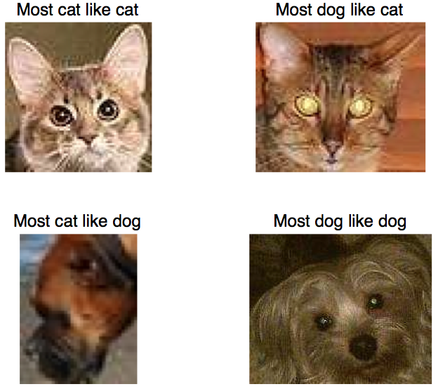
The code also show the most confident confusions like the image below (Note: this will vary too since features are random).
For extra credit
Here are some suggestions for extra credit. You are welcome to come up with your own ideas. The suggestions below are not equally hard, so I've put down relative difficulty of these. You will get more points for implementing something harder.- Other features. Explore other features such as the GIST descriptor from MIT. You will be able to get close to 90% accuracy with this feature and linear SVM. [Difficulty 1]
- Other distance functions. Explore other distance functions such as l1 distance, χ²-distance, etc, in the kNN framework. [Difficulty 1]
- Soft assignment. Instead of hard assignment explore soft assignment schemes, i.e., assign each feature to a number of dictionary items inversely proportional to the distance to them. Explore different functions such as exp(-gamma*distance), 1/distance, 1-distance, etc, and see what works best. For speed you might want to only assign non-zero weights to the k nearest neighbors. The weights should sum up to one for each feature. [Difficulty 1]
- Higher order encodings. You can read about an implement Fisher vectors encodings, a state of the art method in the bag of words framework. If you are using VLFEAT there are inbuilt functions to do this. [Difficulty 3 if using VLFEAT]
- Multi-scale features. Instead of sampling features at a single scale, you could scale the image using a few different values and sample features from all of them. This captures mutli-scale information about the image without increasing the feature dimension. [Difficulty 3]
- Spatial pyramids. Tile up the image into nxn blocks and build a local histogram for each block. Try different values of n and see if it improves performance. To do this you have to keep track of the location of the local features in the sampling step. [Difficulty 3]
Grading checklist
To get full credit for the homework you must:- Report results using tinyimage features using kNN and SVM classifiers and discuss the choices of parameters that worked best. on the validation set. (Accuracy 65-70% on the test set).
- The same for bow-patches features (Accuracy 60-70% on the test set).
- The same for bow-sift features (Accuracy 70-80% on the test set).
- Visualization of the learned dictionary using patches. The code to display is in evalCode.m.
- Show the most confused images on the test set. The last part of the evalCode.m uses the predicted scores to find the most confident correct and incorrect classifications. You should show the output of this step for your most accurate feature with SVM classifier. Note that this can be done only with SVM classifiers as kNN classifiers don't return a score (or confidence) of prediction.
- On what features does kNN work better than SVM. Why?
- The effect of the size of dictionary for patches and SIFT features.
- The effect of other parameter choices.
Instructions for submitting the homework
As before, you must turn in both your report and your code. Your report should include the details and output for each of the Steps listed in this homework.
As before, create a hw5.zip file in your edlab accounts here /courses/cs600/cs670/username/hw5.zip containing the following files:- computeFeatures.m (+ any other code you have written to implement this)
- normalizeFeatures.m
- evalCode.m
- report.pdf
Academic integrity: Feel free to discuss the assignment with each other in general terms, and to search the Web for general guidance (not for complete solutions). Coding should be done individually. If you make substantial use of some code snippets or information from outside sources, be sure to acknowledge the sources in your report. At the first instance of cheating (copying from other students or unacknowledged sources on the Web), a grade of zero will be given for the assignment.
Acknowledgements
Thanks to Oxford and IIIT groups for making the pets dataset publicly available. VLFEAT library is maintained by Andrea Vedaldi. The SIFT implementation included in this homework is written by Svetlana Lazebnik. The SVM solver included in the code is by Olivier Chapelle.