CMPSCI 670: Computer Vision, Fall 2014

Homework 4: Grouping and Texture

Due date: November 5 (before the class starts)

Overview

In this homework you will implement various local image representations for color and texture and use it to segment images and classify materials. For texture you will implement a filter bank and use it to create a texton based representation. The relevant materials for the class are covered in Lectures 10 and 11. You may also find the material in Richard Szeliski's book Chapter 5 useful.

Part 1. Segmentation by grouping

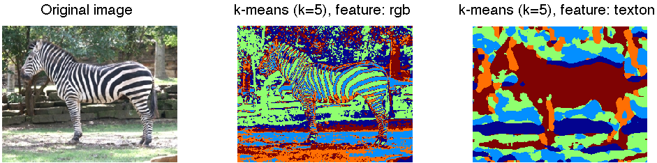
Part 1a. Color based grouping

Although k-means clustering on color alone doesn’t provide very satisfying segmentations, it can be used to reduce the color palette of an image. Implement a function that takes a color image and a value for k and returns a new version of the image which uses only k distinct numbers. Your code should cluster the pixel values using k-means and then produce a new image where each pixel is replaced with index of the closest cluster center. Demonstrate your code on the zebra image for different values of k = 2, 5, 10. Describe what would happen to the clustering if you scale one of the feature coordinates, say the R (red) value by a factor of 100? You can test this by first multiplying the R value by 100 and performing the clustering ~~and then dividing the R value in the result image by 100 prior to displaying it~~. See the code section on how to implement this.

Part 1b. Texture based grouping

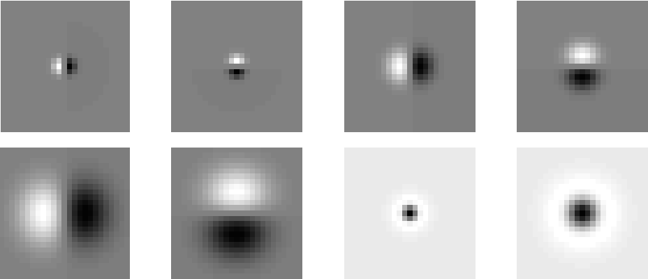
1. Filter outputs: In order to analyze texture, we would like to describe the image in terms of distributions of filter outputs. Implement a filter bank function which takes an image as input and filters the image with Gaussian derivatives in the horizontal and vertical directions at 3 different scales σ = 1, 2, 4. To do this write down the equation of the two dimensional gaussian and take the derivative with respect to x and y. You may find the function meshgrid() useful to generate a 2D grid of x and y values. Also create an additional center surround filter by taking the different of two isotropic Gaussian functions at two different scales, e.g. G2(x, y) − G1(x, y) and G4(x, y) − G2(x, y). Your filterbank function should take as input one grayscale image and return 8 filter response images. Feel free to use the tricks we’ve discussed for making this process fast such as separability. Submit your code and include an image in your writeup which shows your 8 filter kernels. This should be implemented in the function makeFilterbank.m. Your filterbank should roughly resemble the figure below (use showFilterbank.m to display).

2. Texton map: Now cluster this 8 dimensional feature using k-means to 20 clusters and assign each pixel to the identity of the closest cluster center. Include the ouput of this step in your report. You may do this using imagesc(..); colormap jet; functions in MATLAB.

3. Texton histogram: Now aggregate the textons around each pixel within a [2r+1 2r+1] window, setting r=5. This will give you a 20 dimensional histogram representing counts of textons at each pixel. This is the simplest way in which you can capture texture. You could implement this step efficiently by creating 20 binary images and using convolutions for adding up values in a neighborhood. What happens if you make r too large, or small?

4. Texture segmentation: Finally, cluster these 20 dimensional histograms at each pixel using k-means varying the value of k= 2, 5, 10, and show the results. Is your method able to group the region on the body of the zebra into more coherent regions compared to the color based grouping method?

Code

The entry code for this part is in evalSegmentation.m. The current implementation will generate random segmentation. Once you have fully implemented the methods in the script the output should be similar to one shown on top of the page.

Detailed steps:

Implement a filter bank fb=makeFilterbank(). Show the output using showFilterbank(fb).
Implement the function segmentImage(im, param). If you look inside this function it has two steps:
1. feat=computeFeatures(im, param): compute features from the image. This could be simple color values (RGB), or texton histograms. Start with color (Part 1a) features and then implement texton histogram features (Part 1b: Steps 2, 3) in the function textons.m. Remember to convert the image to gray scale and double before you run any convolution operation.
2. seg=groupFeatures(feat, im, param): group features within an image using k-means. See the documentation of how various values of param are passed to the function.

Part 2. Material classification using fiterbank histograms

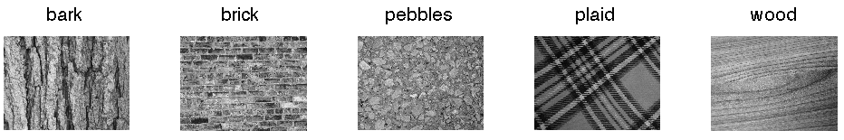
Filterbank histogram: In this part you will use the filterbank responses directly to classify materials. For this dataset we will use a simplified version of UIUC texture database consisting of images from 5 classes namely bark, brick, pebbles, plain and wood. The evalTexture.m has starter code for loading all the images and computing filterbank histograms. To do this use the filterbank you created in the previous step to compute a response over the entire image. Now sum all these values to create a 8 dimensional histograms. Note: you should take the absolute values of the response before computing the histogram. Otherwise the positive and negative values may sum to zero making the texture indistinguishable from uniform texture. You can come up with other ways of representing texture (see the extra credit section).

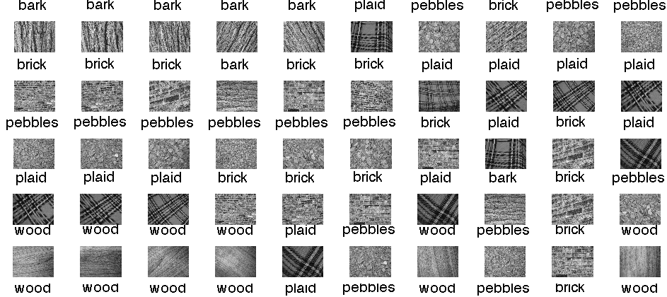
Texture classification: We will test this texture representation for material classification using a simple machine learning method called the "nearest neighbor" algorithm. Given an image we find the closest image in the remaining set using the l2-distance between the histograms and use the label of the nearest neighbor as the prediction. One by one, we hold out an image and count what fraction of the time the nearest neighbor from the remaining set has the same label as the held out image. This measures the accuracy of the nearest neighbour classifier. Aditionally, for each representative image one can also sort all the images in increasing order of the distance and show the top 10 (the first one is itself). This is already implemented in the code. Your output should resemble below, which shows this list for one representative image from each class:

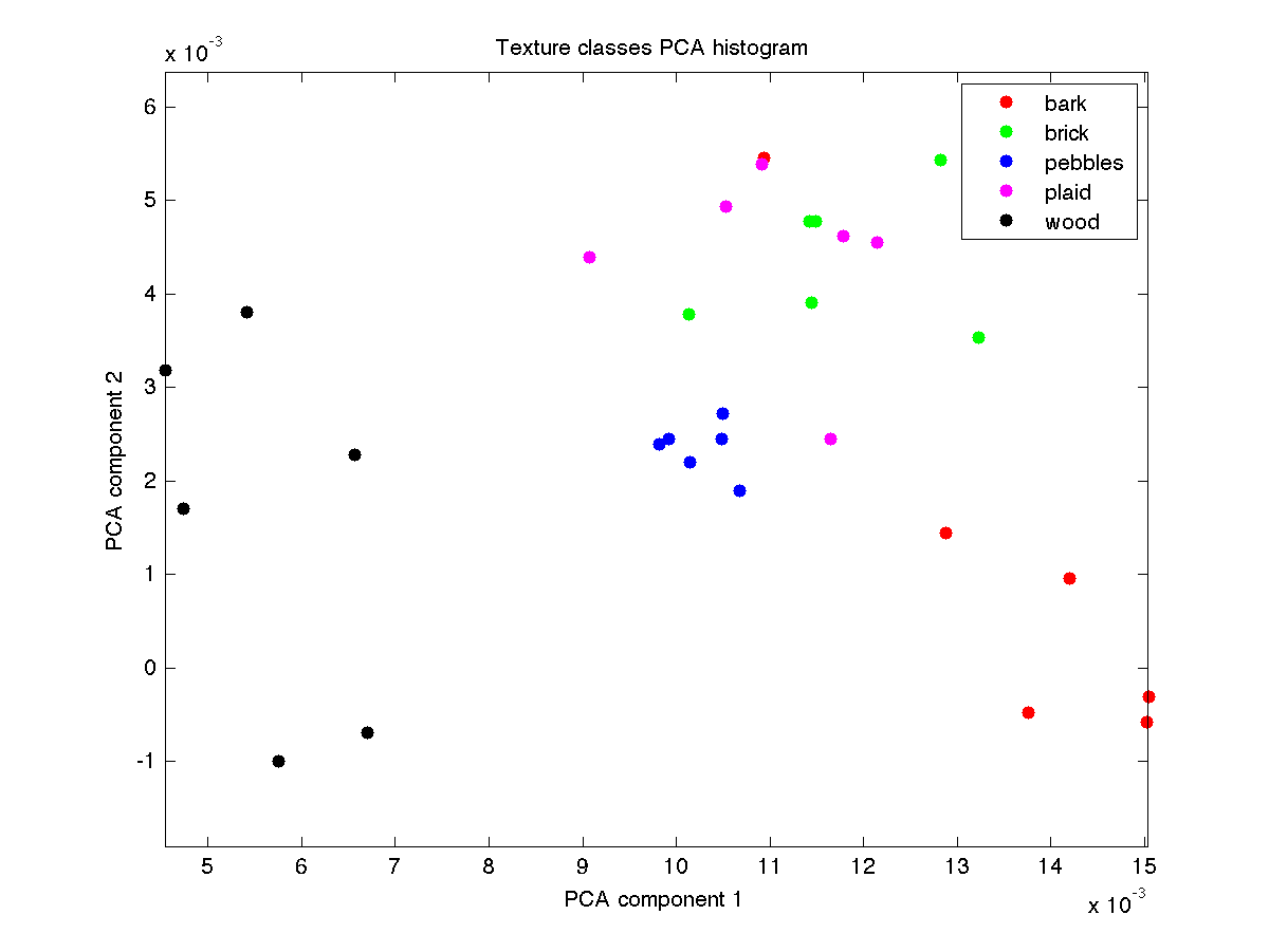
Texture PCA: Another way to visualize the quality of the representation is to perform principal component analysis which finds directions in the data with maximal variation and visualizing the images using the first two components. A good representation will have various classes well separated from each other. This is already implemented in the code. Your output should resemble:

Algorithm outline

Create a filter bank (same as Part 1)
For each image in the dataset:
1. Compute response of the filters, take absolute value.
2. Build a global histogram of these responses.
Use these filterbank histograms for nearest-neighbor classification. Measure accuracy. (Already implemented)
Visualize the classes using the first two components of the PCA of the filterbank histograms. (Already implemented)

Code

All the code for this part is in evalTexture.m. Right now it generates random features and meaningless results. Once you have fully implemented the methods in the script the output will be similar to one shown above and should print the below on the command line:

>> evalTexture
[fbHist 30 images]..............................[done]
Classification accuracy: 86.67%

That is, the method achieves 86.67% accuracy with the representation. The main function you have to implement is the fbHist(i,:) = computeFbHist(im, fb); which computes the filterbank histogram for the i-th image in the database. If implemented correctly the rest of the code should work out of the box.

Detailed steps for implementing computeFbHist(im, fb):

Convert the image to gray scale and double.
Convolve the image with filterbank and take the absolute value of the response.
Compute the total response for each channel and output a histogram

For extra credit

Here are some suggestions for extra credit. You are welcome to come up with your own ideas. The suggestions below are not equally hard, so I've put down relative difficulty of these, so you will get more points for implementing something harder.

Other filter banks: Implement different filter banks and see what the results look for segmentation and material classification. Take a look at the Oxford Visual Geometry Group's webpage which describes various filter banks here. What filterbank performs best for these tasks? [Difficulty 1]
Texton histograms for material classification: In reality instead of texture bank histograms, texton histograms are used for material classification. Texton histograms are similar to the representation used in the texture segmentation part. However the key difference is that instead of using per-image clusters, you have to make sure that the cluster centers are consistent across images. To do this first take 1 image from each category, compute their filter bank responses and cluster all the pixel responses across all images using k-means (k=20). The cluster centers provide a "universal" representation. Now you can use these fixed set of centers to assign filter bank responses to cluster ids across all images. This gives you a 20 dimensional histogram for each image. See if this representation improves performance. [Difficulty 3]
Other image segmentation methods: Implement some other image segmentation method such as "mean shift", or "normalized cuts". Take a look at the relevant material in the slides for this. Both these algorithms are slow, so you might have to use careful data-structures and optimized code to segment images of reasonable size. [Difficulty 4]

Grading checklist

Include the output of color segmentation for k=2, 5, 10. Also include results of scaling the value of R by 100, for the same values of k. Discuss the results.
Show your filterbank using showFilterbank() function. Also include the outputs of convolving the zebra image with the each filter in the filter bank, i.e., 8 images.
Show the output of clustering the filterbank outputs using k-means for k=20. Your output should be an image where each pixel is given a value {1,2,...,20} based on the nearest cluster center (Part 1b. 2).
Discuss the effect of computing texton histograms from various neighbourhood sizes (parameter r, Part 1b. 2) for the final segmentation results. Pick a value of k and vary r and show the results. What is the qualitative effect of changing r?
Show the output of the clustering using k-means the texton histogram representation for k=2, 5, 10 (Part 1b. 4). Discuss the results.
Run evalTexture.m and include in your report the images top10.png and texturePCA.png. Also clearly show the accuracy of the method on the material classification task. Discuss what happens if you did not take the absolute value of the filter response before computing the histograms. What is the accuracy of this method?

Instructions for submitting the homework

As before, you must turn in both your report and your code. Your report should include the details and output for each of the Steps listed in this homework.

As before, create a hw4.zip file in your edlab accounts here /courses/cs600/cs670/username/hw4.zip containing the following files:

segmentImage.m
makeFilterbank.m
computeFeatures.m
groupFeatures.m
textons.m
report.pdf

Note that the result of unzipping the /courses/cs600/cs670/username/hw4.zip should result in files /courses/cs600/cs670/username/hw4/report.pdf, etc. Also include additional code (e.g. for extra credit) and explain it in the report what each file does.

Academic integrity: Feel free to discuss the assignment with each other in general terms, and to search the Web for general guidance (not for complete solutions). Coding should be done individually. If you make substantial use of some code snippets or information from outside sources, be sure to acknowledge the sources in your report. At the first instance of cheating (copying from other students or unacknowledged sources on the Web), a grade of zero will be given for the assignment.

Acknowledgements

This homework is partly based on a similar one made by Charless Flowkes at UC Irvine.