CMPSCI 670: Computer Vision, Fall 2014
Homework 1: Color images
Due date: September 22 (before the class starts)
Overview
In this homework you will learn to manipulate image in MATLAB. Here are some resources about getting started with MATLAB.
This is a two part homework. In the first part you will be coloring historic Prokudin-Gorskii images from intensity measurements of red, green and blue color channels. You must first compute an alignment of the three channels to produce a single color image. In the second part you will implement several demosaicing algorithms to produce color images from Bayer pattern images. This is how digital cameras capture color.
Part 1: Coloring Prokudin-Gorskii images
Sergei Mikhailovich Prokudin-Gorskii was a color photographer far ahead of his time. He undertook a photographic survey of the Russian Empire for Tsar Nicholas II. He was able to capture color pictures by simply taking three pictures of each scene, each with a red, green and blue color filter. There was no way of printing these back in the day, so he envisioned complex display devices to show these. However these were never made, but his pictures survived. In this homework you will reconstruct a color image from his photographs as seen in Figure 1.
The key step to compute the color image is to align the
channels. Alas, since the camera moved between each shot, these
channels are slightly displaced from each other. The simplest way
is to keep one channel fixed say R, and align the G, B channels to
it by searching over displacements in the range [-15, 15] both
horizontally and vertically. Pick the display that maximizes
similarity between the channels. One such measure is dot product,
i.e, R'G. Another is normalized cross-correlation,
which is simply the dot product between l2 normalized R,
G vectors.
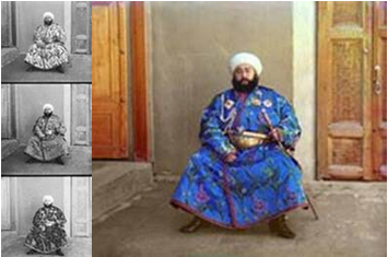
Figure 1: Example image from the Prokudin-Gorskii collection
Before you start aligning the Prokudin-Gorskii images, you will test your code on synthetic images which have been randomly shifted. Your code should correctly discover the inverse of the shift. Note the colors are in B, G, R order from the top to bottom (and not R, G, B)!
Code
Run evalAlignment.m on the MATLAB command prompt inside the code directory. This should produce the
following output.
Note the actual 'gt shift' might be different since it is randomly generated.
    Evaluating alignment ..
    1 balloon.jpeg
	   gt shift: ( 1,11) ( 4, 5)
	 pred shift: ( 0, 0) ( 0, 0)
    2 cat.jpg
	   gt shift: (-5, 5) (-6,-2)
	 pred shift: ( 0, 0) ( 0, 0)
     ...
The code loads a set of images, randomly shifts
the color channels and provides them as input to
alignChannels.m. Your goal is to implement this
function. A correct implementation should obtain the shifts that
is the negative of the ground-truth shifts, i.e., the following
output:
    Evaluating alignment ..
    1 balloon.jpeg
	   gt shift: ( 13, 11)  ( 4, 5)
	 pred shift: (-13,-11)  (-4,-5)
    2 cat.jpg
	   gt shift: (-5, 5) (-6,-2)
	 pred shift: ( 5,-5) ( 6, 2)
     ...
Once you are done with that, run
alignProkudin.m. This will call your function to
align images from the Prokudin-Gorskii collection. The output is
saved to the outDir. Note: if this directory does not exist, you
will have to create it first. In your report, show all the aligned
images as well as the shifts that were computed by your algorithm.
Tips: Look at functions circshift() and
padarray() to deal with shifting images.
Extra credit
Here are some ideas for extra credit:
- Boundary effects: Shifting images causes ugly boundary artifacts. Come up with of a way of avoiding this.
-
Faster alignment: Searching over displacements can be
slow. Think of a way of aligning them faster in a coarse to fine
manner. For example you may align the channels by resizing
them to half the size and then refining the estimate. This can
be done by multiple calls to your
alignChannels()function. -
Gradient domain alignment: Instead of aligning raw
channels, you might want to align the edges to avoid overdue
emphasis on constant intensity regions. You can do this by first
computing an edge intensity image and then using your code to
align the channels. Look at the
edge()function in Matlab.
What to submit?
For this part you have to explain what similarity function
performed the best in your implementation of
alignChannels.m. You have to include the aligned
color images from the output of alignProkudin.m in
the report, as well as, the computed shift vectors for each
image. You also must verify that the evalAlignment.m
correctly recovers the color image and shifts using your code. You
also have to turn in the function alignChannels.m.
Part 2: Color image demosaicing
Recall that in digital cameras the red, blue, and green sensors
are interlaced in a Bayer pattern. Your goal is to fill the
missing values in each channel to obtain a single color image. For
this homework you will implement several different interpolation
algorithms. The input to the algorithm is a single image im, a NxM array of
numbers between 0 and 1. These are measurements in the format shown
in Figure 2, i.e., top left im(1,1) is red, im(1,2)
is green, im(2,1) is green and im(2,2) is
blue channel. Your goal is to create a single
color image C from these measurements.
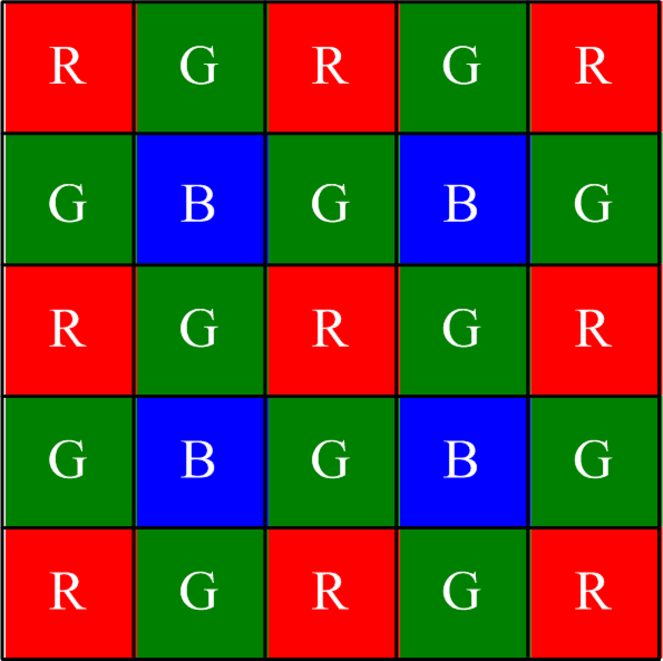
Figure 2: Bayer pattern
Start with some non-adaptive algorithms. Implement nearest neighbour and linear interpolation algorithm. Then implement an adaptive algorithm such as weighted gradient averaging. Compare the results. Where are the errors?
Evaluation
We will evaluate the algorithm by comparing your output to the ground truth color image. The input to the algorithm was constructed by artificially mosaicing it. This is not ideal in practice, since there is a demosacing algorithm that was used to construct the digital image, but we will ignore this for now. We can compute the mean error between each color image and your output and report these numbers for each algorithm.
Code
Run evalDemosaicing on the MATLAB command prompt
inside the code directory. You should be able to see the
output shown in Figure 2. The code loads images from the data directory, artificially mosaics them, and
provides them as input to the demosaicing algorithms. The actual
code for that is in demosaicImage.m file. Right now
only the demosaicImage(im, 'baseline') is implemented. All the other
methods call the baseline methods which is why they produce
identical errors. Your job is to implement the
following functions in the file:
-
demosaicImage(im, 'nn')- nearest-neighbour interpolation. -
demosaicImage(im, 'linear')- linear interpolation. -
demosaicImage(im, 'adagrad')- adaptive gradient interpolation.
The baseline method achieves an average error of 0.1392 across the 10 images in the dataset. Your methods you should be able to achieve substantially better results. As a reference, the linear interpolation method achieves an error of about 0.0174. You should report the results of all your methods in the form of the same table.
----------------------------------------------------------------------------------
# 	 image 		 baseline 	 nn 		 linear 	 adagrad
----------------------------------------------------------------------------------
1 	 balloon.jpeg 	 0.179239 	 0.179239 	 0.179239 	 0.179239
2 	 cat.jpg 	 0.099966 	 0.099966 	 0.099966 	 0.099966
3 	 ip.jpg 	 	 0.231587 	 0.231587 	 0.231587 	 0.231587
4 	 puppy.jpg 	 0.094093 	 0.094093 	 0.094093 	 0.094093
5 	 squirrel.jpg 	 0.121964 	 0.121964 	 0.121964 	 0.121964
6 	 candy.jpeg 	 0.206359 	 0.206359 	 0.206359 	 0.206359
7 	 house.png 	 0.117667 	 0.117667 	 0.117667 	 0.117667
8 	 light.png 	 0.097868 	 0.097868 	 0.097868 	 0.097868
9 	 sails.png 	 0.074946 	 0.074946 	 0.074946 	 0.074946
10 	 tree.jpeg 	 0.167812 	 0.167812 	 0.167812 	 0.167812
----------------------------------------------------------------------------------
 	 average 	 0.139150 	 0.139150 	 0.139150 	 0.139150
----------------------------------------------------------------------------------
Figure 2: Output of
evalDemosaicing.m
Tips: You can visualize at the errors by setting the
display flag to true in the runDemosaicing.m. Avoid loops for
speed in MATLAB. Be careful in handling the boundary of the
images. It might help to think of various operations as
convolutions. Look up MATLAB's conv2() function that
implements 2D convolutions.
Extra credit
Here are some ideas for extra credit:
- Transformed color spaces: Try your previous algorithms by first interpolating the green channel and then transforming the red and blue channels R ← R/G and B ← B/G, i.e., dividing by the green channel and then transforming them back after interpolation. Try other transformations such as logarithm of the ratio, etc (note: you have to apply the appropriate inverse transform). Does this result in better images measured in terms of the mean error? Why is this a good/bad idea?
- Digital Prokudin-Gorskii: Imagine that Prokudin was equipped with a modern digital camera. Compare the resulting demosaiced images to what he obtained using his method of taking three independent grayscale images. Start with the aligned images of your first part and create a mosaiced image by sampling the channels image using the Bayer pattern. Run your demosaicing algorithms and compare the resulting image with the input color image. How much do you lose? Where are the errors?
Writeup
You are required to turn in a writeup describing all the experiments you did. The quality and style of the paper is to be similar to that in a conference paper. We recommend CVPR style sheets, or something similar. The writeup should be self contained, describing the key choices you made. Aim for 2-4 pages with figures etc. Write down any observations you made and try to be as quantitative as possible. This kind of reasoning is critical when you will be writing research papers in your own area. You may also include code snippets, pseudo code, etc. If you do any of the suggested extra credit or your own, explain them clearly, and include any quantitative or qualitative results you obtained, as well as code.
Although, this is the primary way
in which you will be evaluated you are also required to turn in code
for your experiments. For this homework only the functions alignChannels.m and demosaicImage.m should be changed. The output of this method should match those in your report.
Submission
What to submit? To get full credit for this homework you should include the following files in your submission:
- The report as a pdf file.
- Code for part 1, the file
alignChannels.m - Code for part 2, the file
demosaicImage.m
Any extra credit items you have done should also be described in the report and the appropriate code must also be included to recieve full credit.
How to submit the homework
Create a hw1.zip file on the top level directory of your edlab accounts
/courses/cs600/cs670/username/hw1.zip
where hw1.zip contains the following files:
- alignChannels.m
- demosaicImage.m
- report.pdf
Also include additional code (e.g. for extra credit) and explain it in the report what each file does.